Topic: DMD0352

PID Control in Do-more
The basic function of the closed loop process control is to maintain certain process characteristics at desired setpoints. Generally speaking, the process deviates from the desired setpoint reference as a result of load material changes and/or interaction with other elements in the process. The actual condition of the process characteristics (liquid level, temperature, motor speed, etc.) is measured as a process variable (PV) and compared with the target setpoint (SP). When deviations occur, an error is generated, which is the difference between the process variable (actual value) and the setpoint (desired value). Any time an error is detected, the function of the control loop is to modify the control output in order to force the error to back zero.
The following block diagram shows the key parts of a PID control loop. The path from the PLC to the manufacturing process and back to the PLC is the closed loop control.

The Do-more CPU has PID control algorithms which are used to implement a closed loop control system. The Do-more CPU receives a signal from an analog input module (process variable) which is connected to an electronic sensor, such as a thermocouple, pressure transducer, or VFDs, etc. This signal is used by the Closed Loop Controller (PID) instruction to mathematically arrive at the action (control output value) required to keep the process under control.
The following describes the basic PID loop algorithm used in a Do-more CPU. The analog input module receives the process variable in analog form along with an operator entered setpoint; the Do-more CPU computes the error. The error is used in the algorithm computation to provide corrective action at the control output. The function of the control action is based on an output control, which is proportional to the instantaneous error value. The integral control action (reset action) provides additional compensation to the control output, which causes a change in proportion to the value of the change of error over a period of time. The derivative control action (rate change) adds compensation to the control output, which causes a change in proportion to the rate of change of error. These three modes are used to provide the desired control action in Proportional (P), Proportional-Integral (PI), or Proportional-Integral-Derivative (PID) control fashion.
Standard analog input modules are used to interface to field transmitters to obtain the process variable (PV). These transmitters normally provide a 4-20mA current or an analog voltage of various ranges for the control loop. For temperature control, thermocouple or RTD can be connected directly to the appropriate module.
The PID control algorithm receives information from the user program, primarily the control parameters and setpoints. Once the Do-more CPU makes the PID calculation, the result may be used to directly control an actuator connected to a 4-20mA current or voltage output module to move the final control element to make the required change.
Additional ladder logic programming can be added to support both time proportioning (eg. heaters for temperature control) and position actuator (eg. reversible motor on a valve) type of control schemes. The remainder of this chapter will explain how to set up the PID control loop, how to implement the software, and how to tune the loop.
PID Algorithms and Operation
The Proportional–Integral–Derivative (PID) algorithm is widely used in process control. The PID method of control adapts well to electronic solutions, whether implemented in analog or digital components. The Do-more CPU implements the PID equations digitally by solving the basic equations in software. I/O modules serve to convert electronic signals into digital form (or vice versa).
The Do-more CPU uses two types of PID controls: “position” and “velocity”. These terms usually refer to motion control situations, but here we use them in a different sense.
PID Position Algorithm
The control output is calculated so that it responds to the displacement (or position) of the PV from the SP (error term). This is referred to as the ISA / Dependent form of the PID equation. Refer to the following equation:
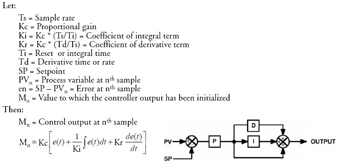
PID Velocity Algorithm
The control output is calculated to represent the rate of change (or velocity) required for the PV to become equal to the SP. Said another way, the Velocity form of the PID equation computes the change in actuator position. This form of the equation is referred to as the velocity PID equation and is obtained by subtracting the equation at time “n” from the equation at time “n-1”. The velocity equation is given by:

The Do-more CPU also combines the integral sum and the initial output into a single term called the bias (Mx). This results in the following set of equations:

By default, the Do-more CPU will keep the normalized output (M) in the range of 0.0 to 1.0. This is done by clamping M to the nearer of 0.0 or 1.0 whenever the calculated output falls outside of this range.
Reset Windup Protection
Reset windup can occur if Reset action (integral term) is specified and the computation of the bias term Mx is:

For example, assume the output is controlling a valve and the process variable (PV) remains at some value greater than the setpoint (SP). The negative error (en) will cause the bias term (Mx) to constantly decrease until the output M goes to 0 closing the valve. However, since the error term is still negative, the bias will continue to decrease becoming more and more negative. When the process variable (PV) finally does come back down below the SP, the valve will stay closed until the error is positive for a long enough time as to cause the bias to become positive again. This will cause the process variable (PV) to undershoot.
To solve this problem the Do-more CPU simply stops changing the bias (also know as Freeze Bias) whenever the computed normalized output (M) falls outside the range of 0.0 to 1.0. This works very well in system where large step changes to the setpoint are anticipated.
Eliminating Proportional, Integral, or Derivative Action
It is not always necessary to run a full three mode PID control loop. Most loops require only the PI terms or just the P term. Parts of the PID equation may be eliminated by choosing appropriate values for the Gain (Kc), Reset (Ti) and Rate (Td) yielding a P, PI, PD, I and even an ID and a D loop.
Eliminating Proportional Action
Although rarely done, the effect of proportional term on the output may be eliminated by setting Kc = 0. Since Kc is also normally a multiplier of the integral coefficient (Ki) and the derivative coefficient (Kr), the CPU makes the computation of these values conditional on the value of Kc as follows:
• Ki = Kc * (Ts / Ti) if Kc <> 0
• Ki = Ts / Ti if Kc = 0 (I only or ID only)
• Kr = Kc * (Td / Ts) if Kc <> 0
• Kr = Td / Ts if Kc = 0 (ID only or D only)
Eliminating Integral Action
The effect of integral action on the output may be eliminated by setting Ti = 0. When this is done, the user may then manually control the bias term (Mx) to eliminate any steady-state offset.
Eliminating Derivative Action
The effect of derivative action on the output may be eliminated by setting Td = 0 (most loops do not require a D parameter; it may make the loop unstable).
Control Output Direction
The Control Output selection in the Closed Loop Controller (PID) instruction designates the relationship between the Output value and the Error value.
A forward Acting Loop drives the output in the same direction as the error, which means that whenever the control output increases, the process variable will also increase.
A Reverse Acting Loop drives the output in the opposite direction from the error, which means that whenever the control output increases, the process variable will decrease.
Bumpless Transfer
The Do-more CPU provides for bumpless mode changes. A bumpless transfer from manual mode to automatic mode is achieved by preventing the control output from changing immediately after the mode change. The bumpless transfer feature of the Do-more CPU is available in two types: Bumpless I and Bumpless II. When a loop is switched from Manual mode to Automatic mode, the setpoint (SP) and Bias (Mx) are initialized as follows:
Bumpless I:
Position PID Algorithm: SP = PV, and Bias (Mx) = Control Output (M)
Velocity PID Algorithm: SP = PV
Bumpless II:
Position PID Algorithm: Bias (Mx) = Control Output (M)
Velocity PID Algorithm: no action
Error Term
The Error Term selection in the Closed Loop Controller (PID) instruction designates optional processing of the Error term. The error will be squared first if both Error Squared and Error Deadband are selected.
A loop with Error Squared enabled is less responsive than a loop using just the error value; however, it will respond faster when the error value is larger, meaning, the smaller the error, the less responsive the loop.
With error deadband control, no control action is taken if the Process Variable (PV) is within the specified deadband area around the setpoint. The error deadband is the same above and below the setpoint. Once the PV is outside of the error deadband around the setpoint, the entire error is used in the loop calculation.
The value for the deadband is set by manipulating the value in <PID reference>.ErrorDB.
Derivative Gain Limit
When the coefficient of the derivative term, Kr, is a large value, noise introduced into the PV can result in erratic loop output. This problem is corrected by specifying a derivative gain limiting coefficient. Derivative gain limiting is a first order filter applied to the derivative term computation. The value for the deadband is set by manipulating the value in <PID reference>.DGainLmt.
Ten Steps to Success
Do-more CPUs provide sophisticated process control features. Automated control systems can be difficult to debug, because a given symptom can have many possible causes. We recommend a careful, step-by-step approach to bringing new control loops online:
Step 1: Know the Recipe
The most important is how to produce your product. This knowledge is the foundation for designing an effective control system. A good process recipe will identify all relevant Process Variables, such as temperature, pressure, or flow rates, etc. which need precise control and plot the desired Setpoint values for each process variables for the duration of one process cycle.
Step 2: Plan Loop Control Strategy
This simply means choosing the method the machine will use to maintain control over the Process Variables to follow their Setpoints. This involves many issues and trade-offs, such as energy efficiency, equipment costs, ability to service the machine during production, and more. You must also determine how to generate the Setpoint value during the process, and whether a machine operator can change the SP.
Step 3: Size and Scale Loop Components
Assuming the control strategy is sound, it is still crucial to properly size the actuator and properly scale the sensors.
Choose an actuator (heater, pump. etc.) which matches the size of the load. An oversized actuator will have an overwhelming effect on your process after a SP change. However, an
undersized actuator will allow the PV to lag or drift away from the SP after a SP change or process disturbance.
Choose a PV sensor which matches the range of interest (and control) for our process. Decide on the resolution of control that you need for the PV (such as 2°C), and make sure the sensor input value provides the loop with at least 5 times that resolution. However, be aware that an overly sensitive sensor can cause control oscillations, etc. The Analog input modules available provide 12-bit, 15-bit and 16-bit, unipolar and bipolar ranges. Which modules you select will affect the SP, PV, Control Output, and Integrator sum.
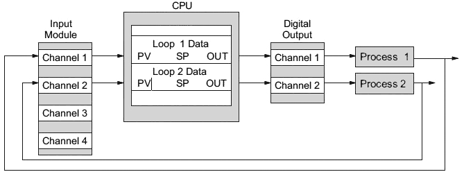
Step 4: Select I/O Modules
After deciding the number of loops, PV variables to measure, and SP values, you can choose the appropriate I/O module. Refer to the figure on the next page. In many cases, you will be able to share input or output modules, or use a analog I/O combination module, among several control loops. The example shows the PV and Control Output signals for two
loops through the same set of modules.
Automationdirect offers analog input modules with 4 channels per module that accept 0 – 20mA or 4 – 20mA signals. Also, analog input and output combination modules are available. Thermocouple and RTD modules can also be used to maintain temperatures to a 10th of a degree. Refer to the sales catalog for further information on these modules, or find the modules on their website, www.automationdirect.com.
Step 5: Wiring and Installation
After selection and procurement of all loop components and I/O module(s), you can perform the wiring and installation. Refer to the wiring guidelines in Chapter 2 of the appropriate User Manual. The most common wiring errors when installing PID loop controls are reversing the polarity of sensor or actuator wiring connections and incorrect signal ground connections between loop components.
Step 6: Loop Parameters
After wiring and installation, choose the loop setup parameters. Do-more Designer provides PID Setup using dialog boxes to simplify the task. Note: It is important to understand the
meaning of all loop parameters mentioned in this chapter before choosing values to enter.
Step 7: Check Open Loop Performance
With the sensor and actuator wiring done, and loop parameters entered, you must manually and carefully check out the new control system using the Manual mode. Verify that the PV value from the sensor is correct. If it is safe to do so, gradually increase the control output up above 0%, and see if the PV responds and moves in the correct direction.
Step 8: Loop Tuning
If the Open Loop Test shows the PV reading is correct and the control output has the proper effect on the process; you can follow the closed loop tuning procedure. In this step, the loop is tuned so the PV automatically follows the SP.
Step 9: Run Process Cycle
If the closed loop test shows the PV will follow small changes in the SP, consider running an actual process cycle. You will need to have completed the programming which will generate the desired SP in real time. In this step, you may want to run a small test batch of product through the machine, watching the SP change according to the recipe.
WARNING: Be sure the Emergency Stop and power-down provision is readily accessible, in case the process goes out of control. Damage to equipment and/or serious injury to personnel can result from loss of control of some processes.
Step 10: Save Parameters
When the loop tests and tuning sessions are complete, be sure to save the project with all of the parameters to disk.
See Also:
PID Control in Do-more
Process Control Instruction Set
Using the PID Process Simulator
Related Topics:
PID Calculation and Tuning Constants
PIDINIT - Set PID Tuning Constants
Alarm Handlers
Input and Output Value Limiters
DEADBAND - Set Outside Deadband
Noise Suppression
INTEGRAT - Integrate Over Time
Ramp/Soak Profiles - up to 250 steps per Profile
Input and Output Scaling
Analog Control using a Discrete Output
TIMEPROP - Time Proportional Control